Azure Data Explorer (ADX) is an outstanding service for continuous ingestion and storage of high velocity telemetry data from cloud services and IoT devices. Leveraging its first-rate performance for querying billions of records, the telemetry data can be further analyzed for various insights such as monitoring service health, production processes, and usage trends. Depending on data velocity and retention policy, data size can rapidly scale to petabytes of data and increase the costs associated with data storage. A common solution for storage of large datasets for a long period of time is to store the data with differing resolution. The most recent data is stored at maximum resolution, meaning all events are stored in raw format. While the historic data is stored at reduced resolution, being filtered and/or aggregated. This solution is often used for time series databases to control hot storage costs.
I’ll use the GitHub events public dataset as the playground. I’ll describe how ADX users can take advantage of stored functions, the “.set-or-append” command, and the Microsoft Flow Azure Kusto connector. This will help you to create and update tables with filtered, down-sampled, and aggregated data for controlling storage costs. The following are steps which I performed.
The ADX demo11 cluster contains a database named GitHub. Since 2016, all events from GHArchive have been ingested into the GitHubEvent table and now total more than 1 billion records. Each GitHub event is represented in a single record with event-related information on the repository, author, comments, and more.



I’ll use the GitHub events public dataset as the playground. I’ll describe how ADX users can take advantage of stored functions, the “.set-or-append” command, and the Microsoft Flow Azure Kusto connector. This will help you to create and update tables with filtered, down-sampled, and aggregated data for controlling storage costs. The following are steps which I performed.
Create a function for down-sampling and aggregation
The ADX demo11 cluster contains a database named GitHub. Since 2016, all events from GHArchive have been ingested into the GitHubEvent table and now total more than 1 billion records. Each GitHub event is represented in a single record with event-related information on the repository, author, comments, and more.

Initially, I created the stored function AggregateReposWeeklyActivity which counts the total number of events in every repository for a given week.
.create-or-alter function with (folder = "TimeSeries", docstring = "Aggregate Weekly Repos Activity”)
AggregateReposWeeklyActivity(StartTime:datetime)
{
let PeriodStart = startofweek(StartTime);
let Period = 7d;
GithubEvent
| where CreatedAt between(PeriodStart .. Period)
| summarize EventCount=count() by RepoName = tostring(Repo.name), StartDate=startofweek(CreatedAt)
| extend EndDate=endofweek(StartDate)
| project StartDate, EndDate, RepoName, EventCount
}
I can now use this function to generate a down-sampled dataset of the weekly repository activity. For example, using the AggregateReposWeeklyActivity function for the first week of 2017 results in a dataset of 867,115 records.

Using Kusto query, create a table with historic data
Since the original dataset starts in 2016, I formulated a program that creates a table named ReposWeeklyActivity and backfills it with weekly aggregated data from the GitHubEvent table. The query runs in parallel ingestion of weekly aggregated datasets using the “.set-or-append” command. The first ingestion operation also creates the table that holds the aggregated data.
.show table GithubEvent details
| project TableName, SizeOnDiskGB=TotalExtentSize/pow(1024,3), TotalRowCount
.show table ReposWeeklyActivity details
| project TableName, SizeOnDiskGB=TotalExtentSize/pow(1024,3), TotalRowCount
Code sample:
using Kusto.Data.Common;
using Kusto.Data.Net.Client;
using System;
using System.Collections.Generic;
using System.Linq;
using System.Text;
using System.Threading.Tasks;
namespace GitHubProcessing
{
class Program
{
static void Main(string[] args)
{
var clusterUrl = "https://demo11.westus.kusto.windows.net:443;Initial Catalog=GitHub;Fed=True";
using (var queryProvider = KustoClientFactory.CreateCslAdminProvider(clusterUrl))
{
Parallel.For(
0,
137,
new ParallelOptions() { MaxDegreeOfParallelism = 8 },
(i) =>
{
var startDate = new DateTime(2016, 01, 03, 0, 0, 0, 0, DateTimeKind.Utc) + TimeSpan.FromDays(7 * i);
var startDateAsCsl = CslDateTimeLiteral.AsCslString(startDate);
var command = $@"
.set-or-append ReposWeeklyActivity <|
AggregateReposWeeklyActivity({startDateAsCsl})";
queryProvider.ExecuteControlCommand(command);
Console.WriteLine($"Finished: start={startDate.ToUniversalTime()}");
});
}
}
}
}
Once the backfill is complete, the ReposWeeklyActivity table will contain 153 million records.

Configure weekly aggregation jobs using Microsoft Flow and Azure Kusto connector
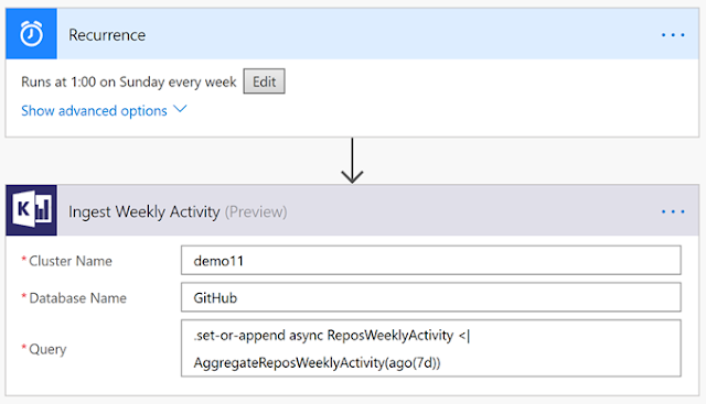
Once the ReposWeeklyActivity table is created and filled with the historic data, we want to make sure it stays updated with new data appended every week. For that purpose, I created a flow in Microsoft Flow that leverages Azure Kusto connector to ingest aggregation data on a weekly basis. The flow is built of two simple steps:
1. Weekly trigger of Microsoft Flow.
2. Use of “.set-or-append” to ingest the aggregated data from the past week.

Start saving
To depict the cost saving potential of down-sampling, I’ve used “.show table <table name> details” command to compare the size of the original GitHubEvent table and the down-sampled table ReposWeeklyActivity.
.show table GithubEvent details
| project TableName, SizeOnDiskGB=TotalExtentSize/pow(1024,3), TotalRowCount
.show table ReposWeeklyActivity details
| project TableName, SizeOnDiskGB=TotalExtentSize/pow(1024,3), TotalRowCount
The results, summarized in the table below, show that for the same time frame the down-sampled data is approximately 10 times smaller in record count and approximately 180 times smaller in storage size.
| Original data | Down-sampled/aggregated data | |
| Time span | 2016-01-01 … 2018-09-26 | 2016-01-01 … 2018-09-26 |
| Record count | 1,048,961,967 | 153,234,107 |
| Total size on disk (indexed and compressed) | 725.2 GB | 4.38 GB |
Converting the cost savings potential to real savings can be performed in various ways. A combination of the different methods are usually most efficient in controlling costs.
◈ Control cluster size and hot storage costs: Set different caching policies for the original data table and down-sampled table. For example, 30 days caching for the original data and two years for the down-sampled table. This configuration allows you to enjoy ADX first-rate performance for interactive exploration of raw data, and analyze activity trends over years. All while controlling cluster size and hot storage costs.
◈ Control cold storage costs: Set different retention policies for the original data table and down-sampled table. For example, 30 days retention for the original data and two years for the down-sampled table. This configuration allows you to explore the raw data and analyze activity trends over years while controlling cold storage costs. On a different note, this configuration is also common for meeting privacy requirements as the raw data might contain user-identifiable information and the aggregated data is usually anonymous.
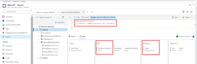
◈ Use the down-sampled table for analysis: Running queries on the down-sampled table for time series trend analysis will consume less CPU and memory resources. In the example below, I compare the resource consumption of a typical query that calculates the total weekly activity across all repositories. The query statistics shows that analyzing weekly activity trends on the down-sampled dataset is approximately 17 times more efficient in CPU consumption and approximately eight times more efficient in memory consumption.
Running this query on the original GitHubEvent table consumes approximately 56 seconds of total CPU time and 176MB of memory.

The same calculation on the aggregated ReposWeeklyActivity table consumes only about three seconds of total CPU time and 16MB of memory.


 Posts
Posts

